Search through your ecological data with the 'grep()' function
(or how to “ctrl-F” your data in R)

We often want to search for a certain character pattern in our data. We do this all the time when we press “ctrl + F” (or “cmd + F” for a mac) on a webpage. For example, maybe you have a list of species names and want to find all of the individuals within a certain genus. Or maybe you have several columns of climate data and only want to select the ones related to precipitation.
Here, I’m going to talk about the functions called grep() and grepl() that allow you to find strings in your data that match the pattern you’re looking for. I’m also going to discuss a function called sub(), which allows you to find and replace strings.
First, let’s load the dplyr package, which I’ll be using once or twice during the tutorial to demonstrate common uses for grep() and grepl(). Note that grep(), grepl(), and sub() come with base R, so there’s no need to load packages to use those functions.
library(dplyr)
Find matches using grep() and grepl()
To demonstrate how to use these functions, I’ve downloaded a data set from the Environmental Data Initiative (EDI) data portal. The EDI archives troves of environmental data that are publicly available and great for demonstration purposes or for supporting your own research. The data I downloaded describe the vegetation on barrier islands within the Virginia Coast Reserve Long-Term Ecological Research project. To follow along, you can download the data here.
Let’s import the data into R and subset it so that it’s easier to understand for this tutorial. I used the select() function in dplyr, where I first listed the data frame I want to analyze, and then the names of the columns I want to keep.
# Upload data
veg_dat <- read.csv("VCR_data.csv")

# Select specific columns
veg_dat <- dplyr::select(veg_dat, genus, species, island, habitat, relabund)

# View first few rows
head(veg_dat)
##      genus     species    island                     habitat relabund
## 1     Acer      rubrum     Smith Pine-Hardwood_forest_stands        6
## 2     Acer      rubrum Parramore      Hardwood_forest_stands        6
## 3 Achillea millefolium     Wreck          Foredune_grassland        3
## 4 Achillea millefolium     Smith      Hardwood_forest_stands        4
## 5 Achillea millefolium     Smith            Dense_grasslands        4
## 6 Achillea millefolium     Smith          Foredune_grassland        4
This data set lists observations of species presence on different islands and in different habitats on those islands. We have a column for genus, species, island, habitat type, and the relative abundance of the species.
Let’s say that we’re interested in looking at all species that are found in forested habitats. How many habitat types do we have that are forested? We can use the unique() function to view all the unique entries for the habitat column.
# View all unique values in the habitat column
unique(veg_dat$habitat)
##  [1] "Pine-Hardwood_forest_stands"
##  [2] "Hardwood_forest_stands"
##  [3] "Foredune_grassland"
##  [4] "Dense_grasslands"
##  [5] "Low_thickets"
##  [6] "Tall_thickets"
##  [7] "Open_dunes-thicket_complex"
##  [8] "Beachgrass_dunes--Dense_grassland_dunes"
##  [9] "Foredune-sparse_grassland_complex"
## [10] "Salt_flat"
## [11] "Sparse_grassland"
## [12] ""
## [13] "Drift--Wrack"
## [14] "Beach"
## [15] "Pine_forest_stands"
## [16] "Fresh_marsh"
## [17] "Upper_salt_marsh"
## [18] "Overwash_flats"
## [19] "Mudflats"
## [20] "Brackish_marsh"
## [21] "Lower_salt_marsh"
## [22] "Pine-hardwood_forest_stands"
## [23] "Juniper_thickets"
## [24] "code_error"
## [25] "Open_water"
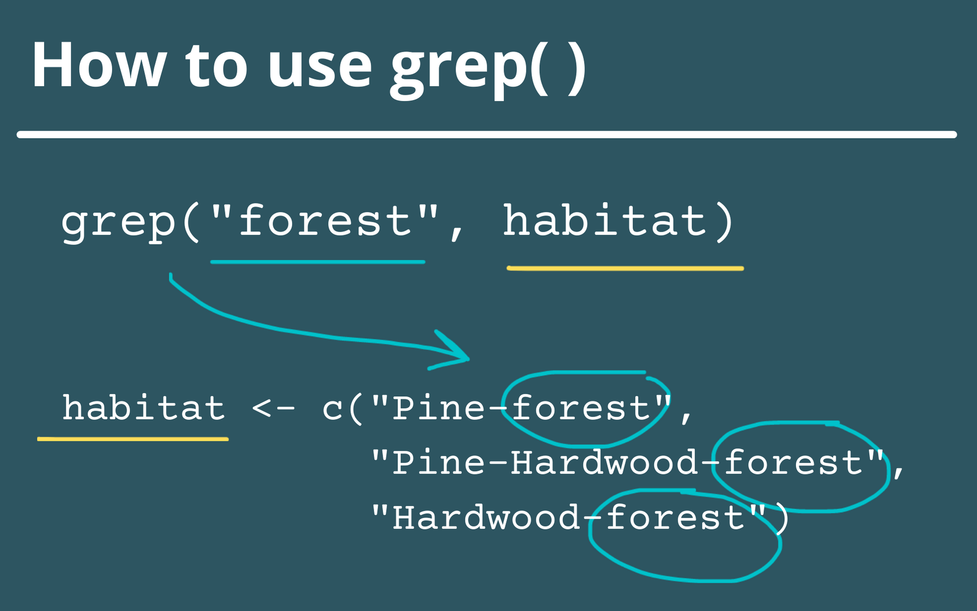
It looks like we have several types of forest: “Pine-Hardwood_forest_stands”, “Hardwood_forest_stands”, and “Pine_forest_stands”. We also have “Pine-hardwood_forest_stands”, which is the same as the first one, but identified as a separate entry because “hardwood” is not capitalized. The easiest way to pick all of these habitats out of the data set would be if we could “ctrl-F” the word “forest” in the habitat column. Luckily, we have the grep() function to help us with that!
You can use the function like so: grep(pattern_text, vector). You can also add an argument to grep() where you set ignore.case = TRUE. This tells the function that you don’t want your search to be case-sensitive (if you leave the ignore.case argument out, the default is that the function is case-sensitive). Let’s try it out.
# Let's see how grep works
grep("forest", veg_dat$habitat, ignore.case = TRUE)
##   [1]    1    2    4    7   34   35   54   91   96   97  106  112  113  114  146
##  [16]  147  152  207  209  218  257  258  259  260  262  263  349  383  384  385
##  [31]  388  389  390  397  398  414  424  442  443  444  474  484  485  488  545
##  [46]  555  558  581  585  595  615  619  750  752  753  754  759  760  762  764
##  [61]  768  771  812  823  828  834  835  837  855  911  915  916  932  933  934
##  [76]  943  944  949  964  965  998 1015 1016 1028 1032 1033 1109 1122 1124 1125
##  [91] 1138 1141 1142 1144 1145 1146 1173 1174 1175 1179 1180 1211 1215 1223 1224
## [106] 1227 1228 1229 1237 1238 1246 1247 1248 1250 1251 1252 1253 1256 1259 1264
## [121] 1265 1269 1270 1271 1272 1288 1289 1300 1408 1410 1458 1459 1462 1463 1464
## [136] 1538 1554 1555 1560 1561 1565 1567 1568 1569 1577 1578 1579 1585 1658 1659
## [151] 1745 1746 1877 1897 1899 1900 1903 1904 1908 1909 1910 1912 1915 1916 1917
## [166] 1918 1922 1923 1930 1931 1951 1952
You can see that grep() returns every row number in the data frame where a habitat type contains the string “forest”. If we add another argument to grep() that says value = TRUE, we can see the values where the function has found a match (in this case, the actual habitat types).
# Assign the list of values to a variable so we don't see them all at once (it's a long list)
hab <- grep("forest", veg_dat$habitat, ignore.case = TRUE, value = TRUE)

# View some of the values
head(hab)
## [1] "Pine-Hardwood_forest_stands" "Hardwood_forest_stands"
## [3] "Hardwood_forest_stands"      "Hardwood_forest_stands"
## [5] "Pine-Hardwood_forest_stands" "Hardwood_forest_stands"
Great! grep() seems pretty useful. So then how does grepl() differ from grep()? The input arguments are the same, but the function gives us a different output. Let’s see:
# Assign the list of values to a variable so we don't have to see all of them (it's a long list)
hab_log <- grepl("forest", veg_dat$habitat, ignore.case = TRUE)

# View the grepl output
head(hab_log, 60)
##  [1]  TRUE  TRUE FALSE  TRUE FALSE FALSE  TRUE FALSE FALSE FALSE FALSE FALSE
## [13] FALSE FALSE FALSE FALSE FALSE FALSE FALSE FALSE FALSE FALSE FALSE FALSE
## [25] FALSE FALSE FALSE FALSE FALSE FALSE FALSE FALSE FALSE  TRUE  TRUE FALSE
## [37] FALSE FALSE FALSE FALSE FALSE FALSE FALSE FALSE FALSE FALSE FALSE FALSE
## [49] FALSE FALSE FALSE FALSE FALSE  TRUE FALSE FALSE FALSE FALSE FALSE FALSE
The extra “l” in grepl() stands for “logical”, which is the data type that it returns. grepl() returns TRUE when there is a match, and FALSE when there isn’t one, all the way down the entire data frame.
Now that we know what grep() and grepl() return, we can subset our data frame using their outputs.
Here, I used grep() to subset the data to return all rows where a species is found in forested habitat.
# Use the grep output to subset the data frame
forest_species <- veg_dat[grep("forest", veg_dat$habitat, ignore.case = TRUE), ]

# View the new data set
head(forest_species)
##          genus     species    island                     habitat relabund
## 1         Acer      rubrum     Smith Pine-Hardwood_forest_stands        6
## 2         Acer      rubrum Parramore      Hardwood_forest_stands        6
## 4     Achillea millefolium     Smith      Hardwood_forest_stands        4
## 7     Achillea millefolium Parramore      Hardwood_forest_stands        5
## 34 Amelanchier    obovalis     Smith Pine-Hardwood_forest_stands        5
## 35 Amelanchier    obovalis     Smith      Hardwood_forest_stands        5
# How many rows?
nrow(forest_species)
## [1] 172
Now I’ll demonstrate the same thing, but this time I’ll use grepl() to subset the data, combined with the filter() function in the dplyr package. The filter() function accepts the name of the data frame you want to analyze, then a logical test. The function will return the rows that are TRUE.
These two methods I demonstrated will return the same data frame, but some prefer to use the filter method as it follows the dplyr methodology for tidy scripts (since it can easily be combined with other functions such as select and mutate. See our post on the pipe operator to learn more).
# Use the grepl output to subset the data frame
forest_species2 <- dplyr::filter(veg_dat, grepl("forest", habitat, ignore.case = TRUE))

# View the new data set
head(forest_species2)
##         genus     species    island                     habitat relabund
## 1        Acer      rubrum     Smith Pine-Hardwood_forest_stands        6
## 2        Acer      rubrum Parramore      Hardwood_forest_stands        6
## 3    Achillea millefolium     Smith      Hardwood_forest_stands        4
## 4    Achillea millefolium Parramore      Hardwood_forest_stands        5
## 5 Amelanchier    obovalis     Smith Pine-Hardwood_forest_stands        5
## 6 Amelanchier    obovalis     Smith      Hardwood_forest_stands        5
# How many rows?
nrow(forest_species2)
## [1] 172
Now that I have a data frame containing only species found in forested habitat, I can do whatever type of data manipulation I want. For example, I could group by island and habitat and use the summarize() function to see how many species are found within each habitat type on each island (to learn more about the group_by() and summarize() functions, check out our tutorial here).
I used the function n() to summarize the data, which just counts the number of rows in each group.
# A dplyr workflow, starting by filtering with grepl(), grouping the data, then summarizing it
forest_summary <- dplyr::filter(veg_dat, grepl("forest", habitat, ignore.case = TRUE)) %>%
  group_by(island, habitat) %>%
  summarize(obs = n())
## `summarise()` has grouped output by 'island'. You can override using the `.groups` argument.
# View summary table
print(forest_summary)
## # A tibble: 8 × 3
## # Groups:   island [3]
##   island    habitat                       obs
##   <chr>     <chr>                       <int>
## 1 Parramore Hardwood_forest_stands         21
## 2 Parramore Pine_forest_stands             27
## 3 Parramore Pine-Hardwood_forest_stands    31
## 4 Revel     Pine-Hardwood_forest_stands     7
## 5 Smith     Hardwood_forest_stands         44
## 6 Smith     Pine_forest_stands              1
## 7 Smith     Pine-hardwood_forest_stands     1
## 8 Smith     Pine-Hardwood_forest_stands    40
Cool! This is useful information to know, and it’s all thanks to grepl() that we were able to perform this operation so easily.
Find and replace using sub()
You may have noticed that the last two rows of the table show that Smith Island has 1 species in “Pine-hardwood_forest_stands”, and 40 species in “Pine-Hardwood_forest_stands”. This is a typo that we need to fix — those two habitat types should be the same.
No worries, we can use the sub() function to replace all instances of “Pine-hardwood_forest_stands” with “Pine-Hardwood_forest_stands”. The function works like this: sub(pattern_text, replacement_text, vector). We’re also going to tell the function ignore.case = F because in this case, we care about the lowercase versus uppercase “H”.
# Substitute all instances of "hardwood" with "Hardwood"
veg_dat$habitat <- sub("hardwood", "Hardwood", veg_dat$habitat, ignore.case = F)
Now if we summarize the data like we did above, all the pine-hardwood forests should be aggregated under the type “Pine-Hardwood_forest_stands”.
# A dplyr workflow, starting by filtering with grepl(), grouping the data, then summarizing it
forest_summary <- dplyr::filter(veg_dat, grepl("forest", habitat, ignore.case = TRUE)) %>%
  group_by(island, habitat) %>%
  summarize(obs = n())
## `summarise()` has grouped output by 'island'. You can override using the `.groups` argument.
# View summary table
forest_summary
## # A tibble: 7 × 3
## # Groups:   island [3]
##   island    habitat                       obs
##   <chr>     <chr>                       <int>
## 1 Parramore Hardwood_forest_stands         21
## 2 Parramore Pine_forest_stands             27
## 3 Parramore Pine-Hardwood_forest_stands    31
## 4 Revel     Pine-Hardwood_forest_stands     7
## 5 Smith     Hardwood_forest_stands         44
## 6 Smith     Pine_forest_stands              1
## 7 Smith     Pine-Hardwood_forest_stands    41
Great! It looks like that fixed the issue.
This was just one example of all the things you could do with grep() and related functions. They’re extremely useful for organizing data and searching for the data you want.
For further reading on strings and how to make your search queries with grep() more specific, learn more about regex (regular expressions) here:
- https://www.rdocumentation.org/packages/base/versions/3.6.2/topics/regex
- https://r4ds.had.co.nz/strings.html
- https://cran.r-project.org/web/packages/stringr/vignettes/regular-expressions.html
I hope you found this tutorial helpful! Happy coding!
Data set citation:
McCaffrey, C. and R. Dueser. 2018. Vegetation Survey on the Virginia Barrier Islands - Species by habitat, 1974 ver 3. Environmental Data Initiative. https://doi.org/10.6073/pasta/9c276fb0ce844030c4afae81ff2cadfb (Accessed 2022-02-25).
Also be sure to check out R-bloggers for other great tutorials on learning R