How to use pipes to clean up your R code

I’ve talked a little bit about pipes (written as %>%) in a past blog post, but they’re so important in R that I thought they deserved their own post.

In this tutorial, I’m going to give an explanation of what pipes are and when they can be used, and then I’m going to demonstrate how useful they can be for writing clean and neat R code.

What is a pipe?

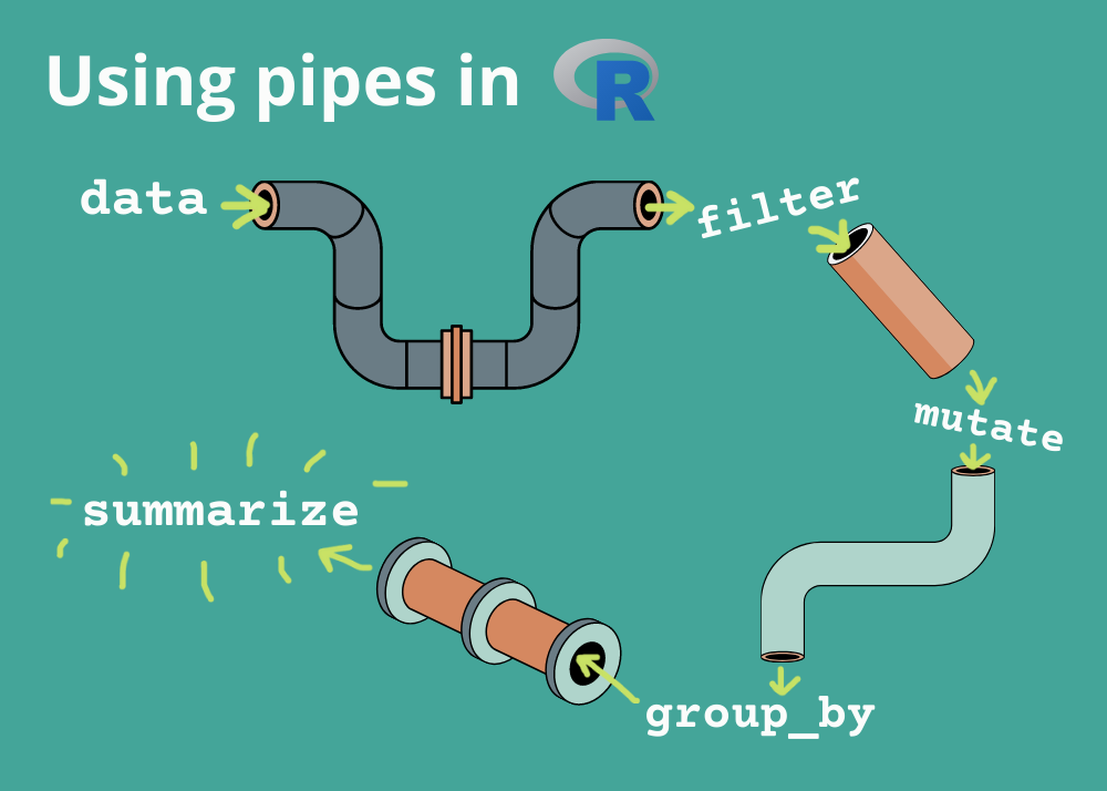
A pipe is a type of operator in R that comes with the magrittr package. It takes the output of one function and passes it as the first argument of the next function, allowing us to chain together several steps in R. Pipes help your code flow better, making it cleaner and more efficient.

The pipe shines when used in conjunction with the dplyr package and its functions such as filter, mutate, and summarise, as we often need to use these one after another to manipulate our data. Luckily, the pipe comes loaded with dplyr, so there’s no need to load the magrittr package unless you specifically need to use the other magrittr operators.

A quick demonstration on how to use pipes

Let’s see pipes in action. First, load the dplyr package and download the classic iris data set that comes with R. If you don’t have dplyr installed yet, you’ll need to run install.packages("dplyr") before loading the package.

# Load dplyr
library(dplyr)

# Load data
data("iris")

# View data
head(iris)

##   Sepal.Length Sepal.Width Petal.Length Petal.Width Species
## 1          5.1         3.5          1.4         0.2  setosa
## 2          4.9         3.0          1.4         0.2  setosa
## 3          4.7         3.2          1.3         0.2  setosa
## 4          4.6         3.1          1.5         0.2  setosa
## 5          5.0         3.6          1.4         0.2  setosa
## 6          5.4         3.9          1.7         0.4  setosa

These data describe several measurements for three plant species (Iris setosa, Iris versicolor, and Iris virginica). These measurements describe morphological differences among the three species in terms of sepal length and width and petal length and width, all in centimeters.

I want to keep only the largest plants in the data set, so let’s only include plants with Sepal.Length greater than 5 cm, and Petal.Length greater than 3 cm. I also want to create two columns called “Sepal.Area” and “Petal.Area”, equivalent to length x width (for an approximation of sepal/petal area). To do this, I’ll use the filter() and mutate() functions. Notice that I also hit “Enter” or “Return” to add a new line after every pipe to keep the code clean and keep each function on a separate line.

# Filter and mutate data
new_iris <- iris %>% 
  filter(Sepal.Length > 5 & Petal.Length > 3) %>%
  mutate(Sepal.Area = Sepal.Length * Sepal.Width,
         Petal.Area = Petal.Length * Petal.Width)

# View new data
head(new_iris)

##   Sepal.Length Sepal.Width Petal.Length Petal.Width    Species Sepal.Area
## 1          7.0         3.2          4.7         1.4 versicolor      22.40
## 2          6.4         3.2          4.5         1.5 versicolor      20.48
## 3          6.9         3.1          4.9         1.5 versicolor      21.39
## 4          5.5         2.3          4.0         1.3 versicolor      12.65
## 5          6.5         2.8          4.6         1.5 versicolor      18.20
## 6          5.7         2.8          4.5         1.3 versicolor      15.96
##   Petal.Area
## 1       6.58
## 2       6.75
## 3       7.35
## 4       5.20
## 5       6.90
## 6       5.85

Our data set looks good. You’ll see that my arguments in the filter() and mutate() functions are a bit different from usual. Normally, most of the dplyr functions are formatted like this: function(data, arguments).

Remember that pipes take the output of what came before it and passes it as the first argument of the function that follows. Thus, the filter() function receives iris as it’s data argument, and then the mutate() function receives filter(data=iris, Sepal.Length > 5 & Petal.Length > 3) as its data argument.

With pipes there was no need for me to write filter(iris, Sepal.Length > 5 & Petal.Length > 3), because that would be repetitive—I could just skip straight to the arguments and write filter(Sepal.Length > 5 & Petal.Length > 3).

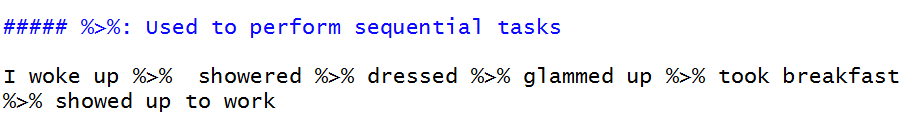
To summarize in plain English (each then in this sentence can be substituted for a pipe):

• I wrote code starting with the iris data set, then filtered it by Sepal.Length and Petal.Length, then used mutate to create two new columns.

Without pipes, our sentence becomes longer:

• I wrote code starting with the iris data set. I filtered the iris data set by Sepal.Length and Petal.Length. Using the filtered iris data, I used mutate to create two new columns.

And those are the essentials of using pipes!

Cleaning code with pipes

After that last example, you might be thinking, OK, that’s pretty cool. But can it really make that big of a difference for organizing my code? The answer is…yes! And I’ll quickly demonstrate why.

Example 1: Creating new variables for each step

Let’s filter and mutate our data like we did above, then group by species and summarize to find the average sepal and petal area within each species. Without pipes, our code might look like this:

filtered_iris <- filter(iris, Sepal.Length > 5 & Petal.Length > 3)
mutated_iris <- mutate(filtered_iris, 
                       Sepal.Area = Sepal.Length * Sepal.Width,
                       Petal.Area = Petal.Length * Petal.Width)
grouped_iris <- group_by(mutated_iris, Species)
summary_iris <- summarize(grouped_iris, 
                          avg.sepal.area = mean(Sepal.Area),
                          avg.petal.area = mean(Petal.Area))

# View result
summary_iris

## # A tibble: 2 × 3
##   Species    avg.sepal.area avg.petal.area
##   <fct>               <dbl>          <dbl>
## 1 versicolor           17.0           5.93
## 2 virginica            19.8          11.4

Whew. It can be a little exhausting to have to save each step as a new variable, and now our environment will be cluttered with a bunch of intermediate variables. Aside from the clutter, your code is also much more prone to errors if you change something in the earlier steps but forget to run those lines before the later steps again. So let’s not do that then.

Example 2: Nesting functions

Let’s try another method, where we nest each function inside the previous one.

summarize(group_by(mutate(filter(iris, 
                                 Sepal.Length > 5 & Petal.Length > 3), 
                          Sepal.Area = Sepal.Length * Sepal.Width,
                          Petal.Area = Petal.Length * Petal.Width), 
                   Species),
          avg.sepal.area = mean(Sepal.Area),
          avg.petal.area = mean(Petal.Area))

## # A tibble: 2 × 3
##   Species    avg.sepal.area avg.petal.area
##   <fct>               <dbl>          <dbl>
## 1 versicolor           17.0           5.93
## 2 virginica            19.8          11.4

That doesn’t really look much better. If all these nested functions are making your head spin, don’t worry, it’s doing that to me too. Code like this is a great way to spend hours searching for errors… only to realize you’re missing a parenthesis. 😖

Example 3: Pipes!

Let’s try it with pipes:

iris %>% 
  filter(Sepal.Length > 5 & Petal.Length > 3) %>%
  mutate(Sepal.Area = Sepal.Length * Sepal.Width,
         Petal.Area = Petal.Length * Petal.Width) %>%
  group_by(Species) %>%
  summarize(avg.sepal.area = mean(Sepal.Area),
            avg.petal.area = mean(Petal.Area))

## # A tibble: 2 × 3
##   Species    avg.sepal.area avg.petal.area
##   <fct>               <dbl>          <dbl>
## 1 versicolor           17.0           5.93
## 2 virginica            19.8          11.4

Now the flow of our code is much cleaner and clearer. Others will be able to follow our code much more easily, and there’s no need to create new variables each step of the way. Pipes take us smoothly from beginning to end.

This way of writing the code also lets us insert comments at each step so we can clearly document our process:

iris %>% 
  # first filter and keep only sepals greater than 5cm long and 3cm wide:
  filter(Sepal.Length > 5 & Petal.Length > 3) %>%
  # then approximate sepal and petal area by multiplying length and width:
  mutate(Sepal.Area = Sepal.Length * Sepal.Width,
         Petal.Area = Petal.Length * Petal.Width) %>%
  # after that group by species to summarize the mean 
  # sepal/petal area of each species:
  group_by(Species) %>%
  summarize(avg.sepal.area = mean(Sepal.Area),
            avg.petal.area = mean(Petal.Area))

## # A tibble: 2 × 3
##   Species    avg.sepal.area avg.petal.area
##   <fct>               <dbl>          <dbl>
## 1 versicolor           17.0           5.93
## 2 virginica            19.8          11.4

All that said, I’m not suggesting that your entire R analysis script fit inside one long set of pipes. Find what works best for you and your analyses in terms of splitting up your code into neat organized chunks that make sense.

We owe a big thank you to Stefan Milton Bache (@stefanbache on Twitter), creator of the magrittr package and the almighty pipe! Hope you found this tutorial helpful. Happy coding!

P.S. A highly relevant tweet explaining pipes… (from WeAreRLadies on Twitter)