How to join tables in R

In this blog post, I’m going to talk about joining data tables together. Joining tables is incredibly useful when you have to download several data files on a common set of subjects and then aggregate them into a larger, singular data set.

This is pretty common with spatial data. For example, you might have one table that contains geographic information on parcels of land like census tracts, each with their own ID. You can then find separate demographic or economic data tables online that can link up with the geographic data using the census tract ID.

Another common example is if you collected community survey data from plots, but then also have associated environmental data collected from those same plots saved as a different spreadsheet of data.

These kinds of situations would call for you to merge, or join, your two data tables together. In this tutorial, I’m going to introduce you to different types of joins, and I’ll show you how to perform joins both in base R and using the dplyr package.

Joining data in base R

We’re going to start with a basic data set. These data contain 6 different students and the distance of their morning commute to school, in miles.

# Create a data frame with information on where students live
set.seed(123)
student_residence <- data.frame(student = seq(1, 6), 
                                distance = runif(6, 3, 10))

# Look at the data
head(student_residence)

##   student distance
## 1       1 5.013043
## 2       2 8.518136
## 3       3 5.862838
## 4       4 9.181122
## 5       5 9.583271
## 6       6 3.318895

The runif() function creates a random assortment of numbers between a minimum and maximum value that you specify. I asked runif() to generate 6 random numbers between 3 and 10. The set.seed() function just makes it so that each time you run this code, the random output will always be the same (when using the same seed number). Use set.seed(123) if you’d like to follow along with the same numbers I have here.

Students at this school were also surveyed to find out what method of transportation they use to get to school in the morning. This survey was offered to several students, but not everyone responded (looks like only students 1, 3, 5, and 7 responded). Note that in this scenario we somehow don’t have data on commute distance for student 7.

# Create another data frame with information on how students get to school
student_transport <- data.frame(student = seq(1, 7, by = 2), 
                                transport = c("Bus", "Carpool", "Walk", "Bus"))

# Look at the data
head(student_transport)

##   student transport
## 1       1       Bus
## 2       3   Carpool
## 3       5      Walk
## 4       7       Bus

Let’s say we want to look at both student transportation methods and morning commute distance so we can create a better bus schedule. It’s tough to do that when transportation method and commute distance are in different data sets, so we want to join them together.

Importantly, to join two different tables together, you need to make sure you have a column in common between both data sets. This common column is called a “key”, and it should provide a unique identifier for every row. In the case of our data, the “student” column is our key, and it provides a unique number for each student.

To join our data, we can use the merge() function in base R. merge() will first accept two data frames as arguments, and then the name of the column that the two data frames have in common, like so: merge(x = dataframe1, y = dataframe2, by = "column name"). With our data, this would look like:

# Merge data frames together
students <- merge(x = student_residence, y = student_transport, by = "student")

If we compare the values for student 1 in the new and old data sets, the values are the same. Great! Looks like the merge worked.

# Compare the data to see if the merge worked
head(students)

##   student distance transport
## 1       1 5.013043       Bus
## 2       3 5.862838   Carpool
## 3       5 9.583271      Walk

student_residence[1, 2]

## [1] 5.013043

student_transport[1, 2]

## [1] "Bus"

But what if the common columns that we want to merge by don’t have the same name? Let’s change the name of the “student” column in student_transport to “studentID” instead.

# View data
head(student_transport)

##   studentID transport
## 1         1       Bus
## 2         3   Carpool
## 3         5      Walk
## 4         7       Bus

If this is the case, we can still use the merge() function with the names of two data frames, but instead of using one “by” argument, we’re going to use two, the by.x() and by.y() arguments, like so: merge(x = dataframe1, y = dataframe2, by.x = "dataframe1 column", by.y = "dataframe2 column").

# Try the merge again
students2 <- merge(x = student_residence, y = student_transport, by.x = "student", by.y = "studentID")

# Compare this new data set to the old one
head(students2)

##   student distance transport
## 1       1 5.013043       Bus
## 2       3 5.862838   Carpool
## 3       5 9.583271      Walk

head(students)

##   student distance transport
## 1       1 5.013043       Bus
## 2       3 5.862838   Carpool
## 3       5 9.583271      Walk

The data sets look the same, so we know both methods worked.

Types of Joins

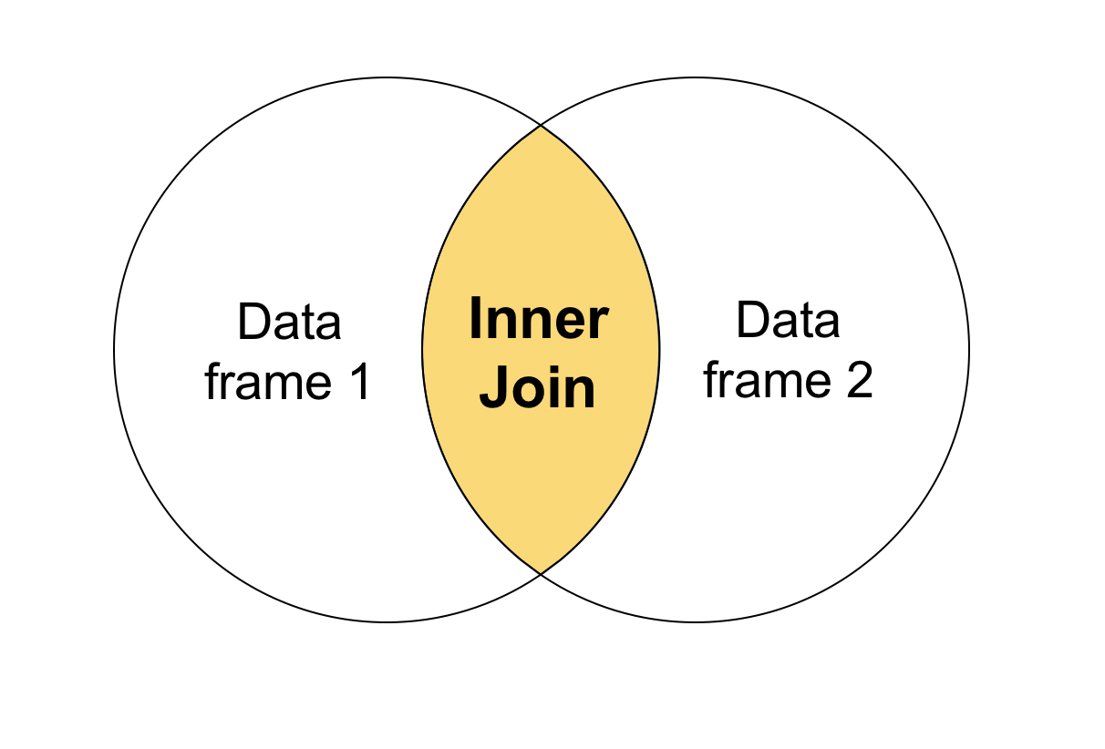
Inner join

You probably noticed that in the join we just performed, there were only three rows in the joined table. That’s because we performed something called an “inner join”, where R only returns the data frame rows that match up with the other data frame. If you were to visualize this type of join, it would look something like this:

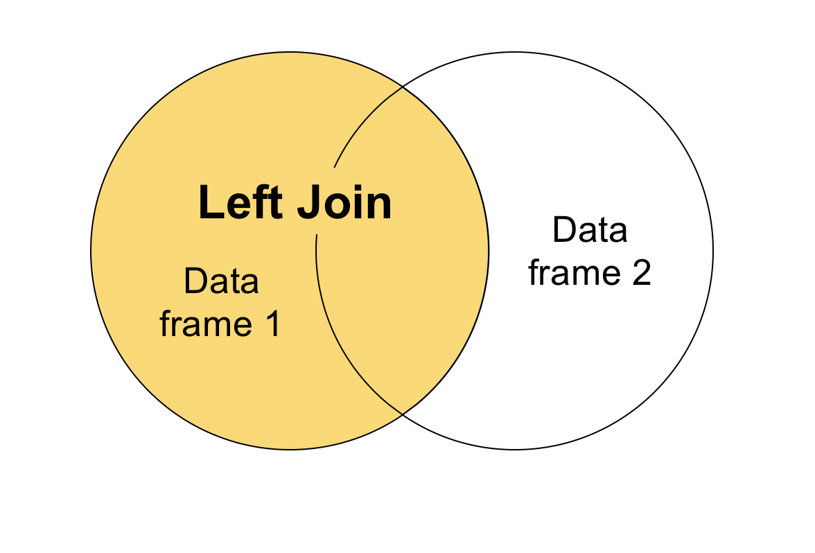
Left join

There are also “left” joins and “right” joins. A left join returns all rows from the left data frame and any matching rows from the right data frame. In the merge() function, the “left” data frame is the x data frame, or the one you name first. The “right” data frame is the y data frame, or the one you list second. We can tell merge() that we want to keep all rows from the “left” data frame by adding the argument all.x = TRUE. If we’re more interested in where students live, we’ll want to keep all the rows from student_residence. Let’s go ahead and do that:

# Perform a left join
merge(x = student_residence, y = student_transport, by = "student", all.x = T)

##   student distance transport
## 1       1 5.013043       Bus
## 2       2 8.518136      <NA>
## 3       3 5.862838   Carpool
## 4       4 9.181122      <NA>
## 5       5 9.583271      Walk
## 6       6 3.318895      <NA>

We can see that indeed, all the rows from student_residence have been kept. Since student_transport was missing some of the student records, there are NAs in the table where the join operation couldn’t find a match for the student. The image below visualizes what a left join would look like.

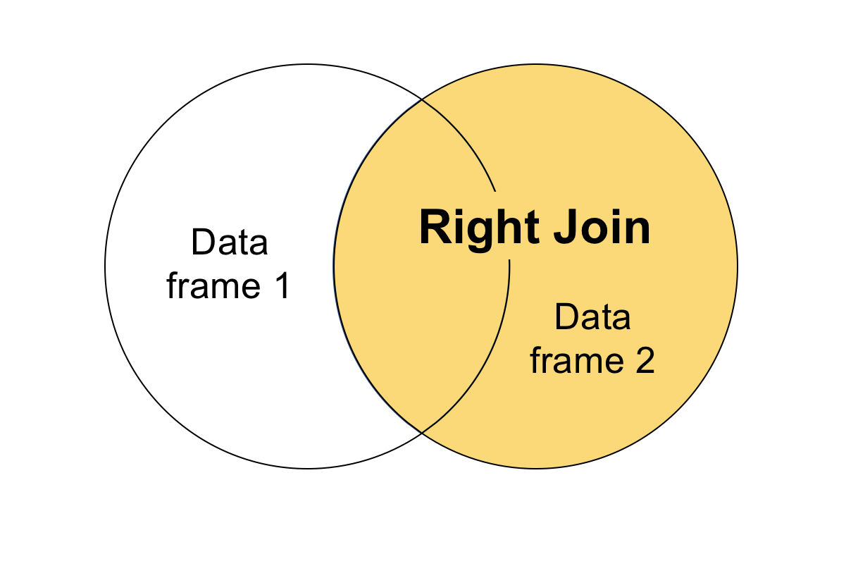
Right join

A right join does the same thing as a left join, just swapping the arguments. Instead of specifying all.x, we’ll use the argument all.y = TRUE. If we’re more interested in student transportation methods, we’ll want to keep all the rows from student_transport.

# Perform a right join
merge(x = student_residence, y = student_transport, by = "student", all.y = T)

##   student distance transport
## 1       1 5.013043       Bus
## 2       3 5.862838   Carpool
## 3       5 9.583271      Walk
## 4       7       NA       Bus

Now, we have all the rows from student_transport. Again, there’s an NA where the join operation couldn’t find a match for the student in the other data frame. The image below visualizes what a right join does.

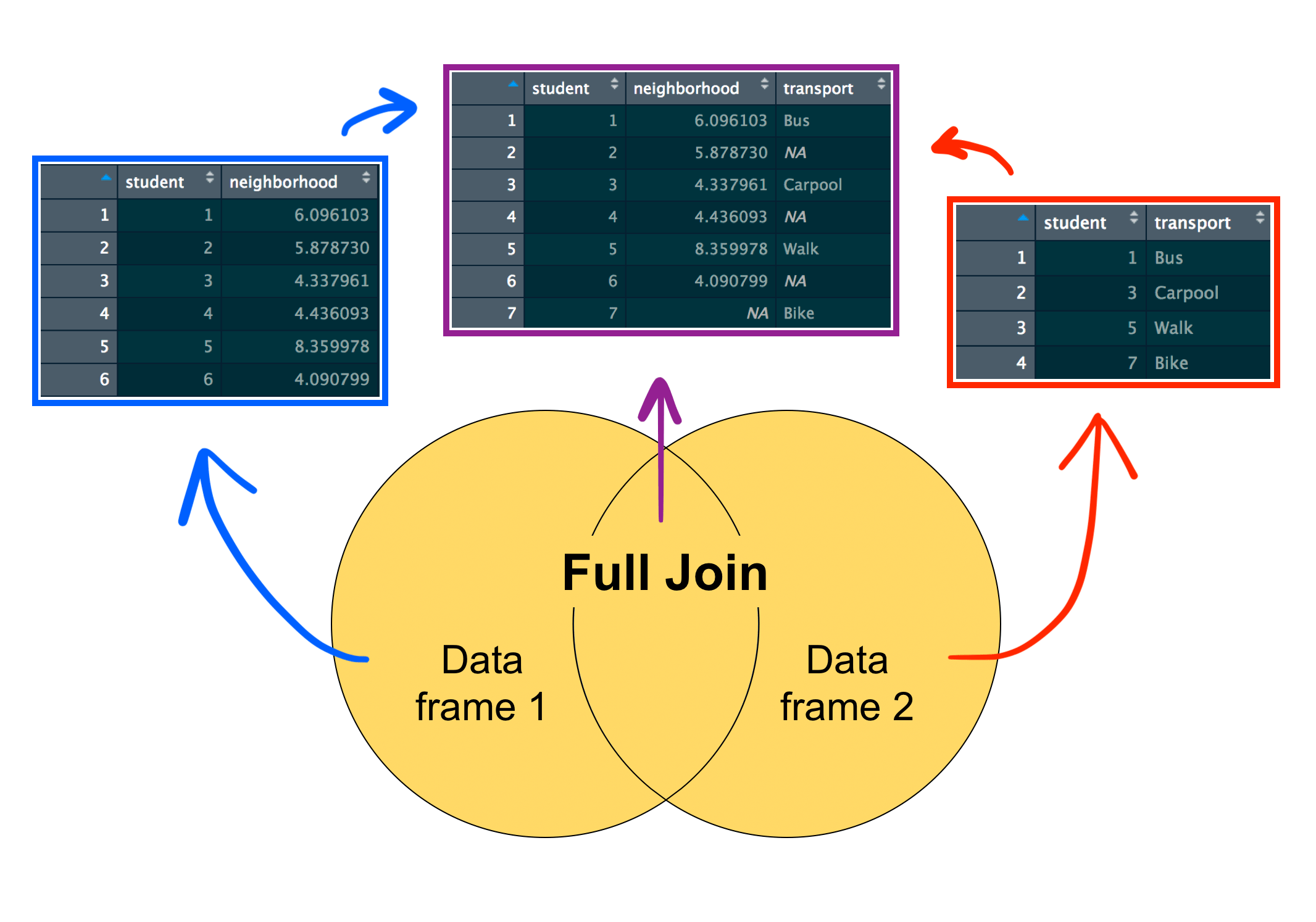
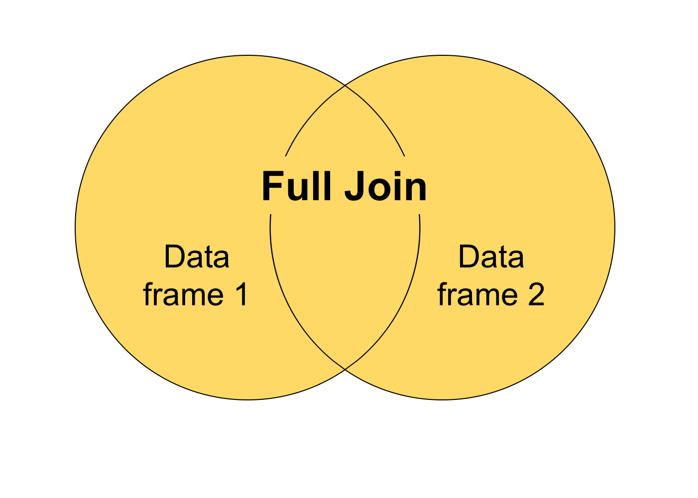
Full join

The last type of join is called a “full join” (or “outer join”) which includes all the rows from both data frames, whether or not they match with one another. We can specify this by including both the all.x and all.y arguments.

# Perform a full join
merge(x = student_residence, y = student_transport, by = "student", all.x = T, all.y = T)

##   student distance transport
## 1       1 5.013043       Bus
## 2       2 8.518136      <NA>
## 3       3 5.862838   Carpool
## 4       4 9.181122      <NA>
## 5       5 9.583271      Walk
## 6       6 3.318895      <NA>
## 7       7       NA       Bus

Joining data using the dplyr package

I just demonstrated how to join tables in base R, but many of you are probably also familiar with the dplyr package. dplyr provides a convenient way to perform the different types of joins using the functions inner_join(), left_join(), right_join(), and full_join(). All of these functions accept the forms XXX_join(dataframe1, dataframe2, by = "column name"), and you don’t need to add anything else like all.x or all.y because the specific type of join is already built into the specific function. I’ll quickly demonstrate how to use these functions below:

# Load package
library(dplyr)

# Inner join
inner_join(student_residence, student_transport, by = "student")

##   student distance transport
## 1       1 5.013043       Bus
## 2       3 5.862838   Carpool
## 3       5 9.583271      Walk

# Left join
left_join(student_residence, student_transport, by = "student")

##   student distance transport
## 1       1 5.013043       Bus
## 2       2 8.518136      <NA>
## 3       3 5.862838   Carpool
## 4       4 9.181122      <NA>
## 5       5 9.583271      Walk
## 6       6 3.318895      <NA>

# Right join
right_join(student_residence, student_transport, by = "student")

##   student distance transport
## 1       1 5.013043       Bus
## 2       3 5.862838   Carpool
## 3       5 9.583271      Walk
## 4       7       NA       Bus

# Full join
full_join(student_residence, student_transport, by = "student")

##   student distance transport
## 1       1 5.013043       Bus
## 2       2 8.518136      <NA>
## 3       3 5.862838   Carpool
## 4       4 9.181122      <NA>
## 5       5 9.583271      Walk
## 6       6 3.318895      <NA>
## 7       7       NA       Bus

# Inner join but if your data frames have different column names
colnames(student_transport)[1] <- "studentID"
inner_join(student_residence, student_transport, by = c("student" = "studentID"))

##   student distance transport
## 1       1 5.013043       Bus
## 2       3 5.862838   Carpool
## 3       5 9.583271      Walk

These joins should look the same as the ones demonstrated above using the merge() function. And now you know how to perform several types of join operations depending on which rows you need to retain!

I hope this tutorial was helpful! Let us know what other tutorials you’d like to see in the comments below. 👇