How to do a simple linear regression in R

In this tutorial I show you how to do a simple linear regression in R that models the relationship between two numeric variables.

Check out this tutorial on YouTube if you’d prefer to follow along while I do the coding:

The first step is to load some data. We’ll use the ‘trees’ dataset that comes built in with R:

# Load the data:
data(trees)

# Show the top few entries:
head(trees)

##   Girth Height Volume
## 1   8.3     70   10.3
## 2   8.6     65   10.3
## 3   8.8     63   10.2
## 4  10.5     72   16.4
## 5  10.7     81   18.8
## 6  10.8     83   19.7

These data include measurements of the diameter, height and volume of 31 black cherry trees. Note that the ‘Girth’ is actually the diameter at breast height (DBH) in inches, ‘Height’ is height in feet, and ‘Volume’ is volume in cubic feet. So let’s just rename those variable names for clarity:

# rename columns
names(trees) <- c("DBH_in","height_ft", "volume_ft3")

head(trees)

##   DBH_in height_ft volume_ft3
## 1    8.3        70       10.3
## 2    8.6        65       10.3
## 3    8.8        63       10.2
## 4   10.5        72       16.4
## 5   10.7        81       18.8
## 6   10.8        83       19.7

There we go.

Now, for the basic linear regression, let’s model how the tree diameters change as they grow taller.

First, let’s start by writing out what it is we actually want to model. We want to know how DBH varies as a function of tree height, but we can also write that out as: DBH_in ~ height_ft, the tilde (~) being read as “is a function of.”

You can also think of this as the Y variable (the dependent or response variable) is a function of the X variable. How does Y depend on or respond to X?

Now let’s visualize the potential association of these variables by plotting our model. The neat thing is that we can write out the plotting function using our “is a function of” notation:

plot(DBH_in ~ height_ft, data = trees, pch=16)

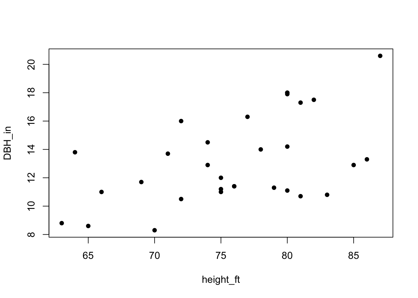
I’m not a fan of the open circle points, so I added in the argument ‘pch = 16’ to that plotting function to fill in the circles.

So there appears to be a trend of increasing DBH with increasing height, but is that trend statistically significant?

To test that, we will use the function lm(), which stands for linear model. The syntax is actually almost exactly the same as our plot! The only difference is that we will save the output of the model to its own object called ‘mod’:

# Run the linear model and save it as 'mod'
mod <- lm(DBH_in ~ height_ft, data = trees)

# let's view the output:
mod

## 
## Call:
## lm(formula = DBH_in ~ height_ft, data = trees)
## 
## Coefficients:
## (Intercept)    height_ft  
##     -6.1884       0.2557

If we look at ‘mod’ we don’t get much to work with, just the coefficient estimates for the intercept and slope. But we can run the ‘summary’ function with ‘mod’ to get more interesting results:

summary(mod)

## 
## Call:
## lm(formula = DBH_in ~ height_ft, data = trees)
## 
## Residuals:
##     Min      1Q  Median      3Q     Max 
## -4.2386 -1.9205 -0.0714  2.7450  4.5384 
## 
## Coefficients:
##             Estimate Std. Error t value Pr(>|t|)   
## (Intercept) -6.18839    5.96020  -1.038  0.30772   
## height_ft    0.25575    0.07816   3.272  0.00276 **
## ---
## Signif. codes:  0 '***' 0.001 '**' 0.01 '*' 0.05 '.' 0.1 ' ' 1
## 
## Residual standard error: 2.728 on 29 degrees of freedom
## Multiple R-squared:  0.2697,	Adjusted R-squared:  0.2445 
## F-statistic: 10.71 on 1 and 29 DF,  p-value: 0.002758

Beneath ‘Call’ and where it shows us what our model looks like, we can see the distribution of the residuals or unexplained variance in our model: the min and max, the 1st and 3rd quartiles, and the median.

But below that we have a table that gets a bit more interesting…

Remember that two coefficients get estimated from a basic linear model: The intercept and the slope. To model a line, we use the equation Y = a + bX, and the goal of the regression analysis is to estimate the a and the b.

In that first column we have that estimate for each coefficient. Then we have the standard error of those estimates, then the test statistic, and finally, the p-value of each coefficient, which tests whether the intercept or slope values are actually zero. In our case, the p-value for the slope (height_ft) coefficient is less than 0.05, allowing you to say that the association of DBH_in and height_ft is statistically significantly.

To make reading these results a bit easier, the this model summary output also includes asterisk symbols that indicate the significance levels of the p-values.

Continuing to go down the summary we can see the residual standard error, and then we have the multiple R squared, or simply R². This can thought of as the proportion of variance in the data explained by the model. You can ignore the adjusted R squared for now if you are just starting out.

Finally we have the F-statistic and p-value testing whether all coefficients in the model are zero.

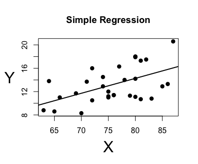
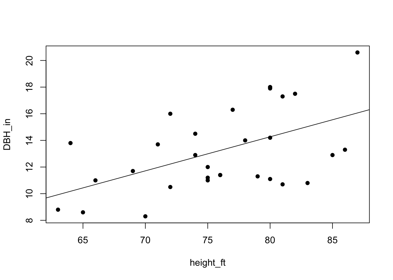
Next we’ll add a line to our plot that shows the fitted line from this model.

All you have to do is first run the plot function that we ran before, and then run the ‘abline’ function with the model as it’s argument:

# Plot the scatterplot as before:
plot(DBH_in ~ height_ft, data = trees, pch=16)

# And then plot the fitted line:
abline(mod)

Finally, you might need to extract a table with the regression results from the summary output, so I’ll show you a quick trick for doing that easily using the ‘broom’ package.

First, make sure to install the broom package if you haven’t already (though you only have to do this once for your computer), and then run the ‘library’ function to load up that package (you have to do this each time you open up R and start a new working session):

# Install the 'broom' package:
# install.packages('broom') #commented out since I already have it installed

# Then load the package:
library('broom')

Finally, use the ‘tidy’ function to extract the table of results from your model:

# extract the table
my_results <- tidy(mod)

my_results

## # A tibble: 2 × 5
##   term        estimate std.error statistic p.value
##   <chr>          <dbl>     <dbl>     <dbl>   <dbl>
## 1 (Intercept)   -6.19     5.96       -1.04 0.308  
## 2 height_ft      0.256    0.0782      3.27 0.00276

And that’s it!